A vibration example with two modes

In the following example, we explore the a mechanical vibration example, especially with regard to its modes of vibration. Both undamped and (under)damped cases are considered and we discover the effects of damping.

Example 7.3

Consider the system of figure 7.3 in which a velocity source V_S is applied to spring K₁, which connects to mass m₁, which in turn is connected via spring K₂ and damper B to mass m₂ which.¹

Figure 7.3: Schematic of the two-mass system.

The state-space model A-matrix is given as $$\begin{aligned} A &= \begin{bmatrix} -B/m_1 & -1/m_1 & B/m_1 & 0 \\ K_1 & 0 & -K_1 & 0 \\ B/m_2 & 1/m_2 & -B/m_2 & -1/m_2 \\ 0 & 0 & K_2 & 0 \end{bmatrix} \end{aligned}$$ with parameters as follows:

m₁ = 0.1 kg
m₂ = 1.1 kg
K₁ = 8 N/m
K₂ = 9 N/m

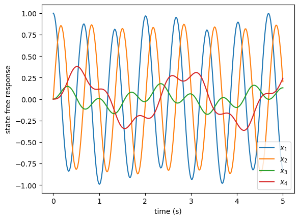
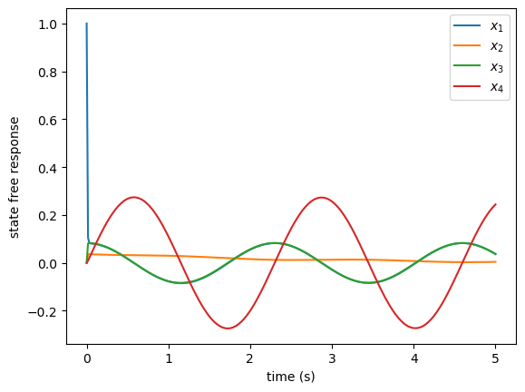
Two different values for B will be considered: 0 and 20 N⋅s/m. We will explore the modes of vibration in each case and plot a corresponding free response.

This common situation appears in a slightly modified form in @Rowell1997.↩︎

Setting up the problem

We analyze the problem with Python. First, we load packages for symbolic, numeric, and graphical analysis, as follow:

import sympy as sp
import numpy as np 
import matplotlib.pyplot as plt
from pprint import pprint

The A matrix is first defined symbolically.

sp.var("m_1, m_2, K_1, K_2, B", real=True)
A = sp.Matrix([
  [-B/m_1, -1/m_1, B/m_1, 0],
  [K_1, 0, -K_1, 0],
  [B/m_2, 1/m_2, -B/m_2, -1/m_2],
  [0, 0, K_2, 0]
])

Now define dictionaries for the parameter values.

p = {
    m_1: 0.1, # kg
    m_2: 1.1, # kg
    K_1: 8,   # N/m
    K_2: 9    # N/m
}
pB1 = {B: 0}  # N/(rad/s), without damping
pB2 = {B: 20} # N/(rad/s), with damping

Without damping

Without damping, we expect the system to be marginally stable and have two pairs of second-order undamped subsystems with their own unique natural frequencies. The numerical A matrix can be computed by substituting in the parameters in p and pB1, as follows:

A_1 = np.array(A.subs(p).subs(pB1), dtype=float)
print(A_1)

[[  0.         -10.           0.           0.        ]
 [  8.           0.          -8.           0.        ]
 [  0.           0.90909091   0.          -0.90909091]
 [  0.           0.           9.           0.        ]]

To explore the modes of vibration, we consider the eigendecomposition of A.

l_,M_ = np.linalg.eig(A_1)
thr = 1e-14                       # threshold for calling something 0
l_.real[abs(l_.real) < thr] = 0.0 # zeroing small real parts

Let’s take a closer look at the eigenvalues.

print(l_)

[0.+9.38179379j 0.-9.38179379j 0.+2.726993j   0.-2.726993j  ]

So we have two pairs of purely imaginary eigenvalues. We would say, then, that there are two “modes of vibration,” and similarly two second-order systems comprising this fourth-order system. When we consider what the natural frequency and damping ratio is for each pair, we’re considering the natural frequencies associated with each “mode of vibration.”

For a second-order system (see ), the roots of the characteristic equation, which are equal to the eigenvalues corresponding to that second-order pair, are given in terms of natural frequency ω_n and damping ratio ζ: $$\maybeeq{ \begin{equation*} -\omega_n\zeta \pm \omega_n \sqrt{\zeta^2-1}. \end{equation*} }$$

So the imaginary part is nonzero only when ζ ∈ [0, 1), that is, when the system is underdamped or undamped. In this case, $$\maybeeq{ \begin{equation} -\omega_n\zeta \pm j \omega_n \sqrt{1-\zeta^2}. \end{equation} }$$

This, taken with the fact that the eigenvalues in l_ have zero real parts, implies either ω_n or ζ is zero. But if ω_n is zero, the eigenvalues would all be zero, which they are not. Therefore, ζ = 0 for both pairs of eigenvalues.

This leaves us with eigenvalues: ± jω_n₁ and ± jω_n₂.

So we can easily identify the natural frequencies ω_n₁ and ω_n₂ associated with each mode as follows.

wn_1 = np.imag(l_[0]);
wn_2 = np.imag(l_[2]);
print(f"Natural frequencies (rad/s): {wn_1} and {wn_2}")

Natural frequencies (rad/s): 9.38179378603641 and 2.726992997943728

Free response

Let’s compute the free response to some initial conditions. The free state response is given by $$\maybeeq{ \begin{align*} \bm{x}(t) = \Phi(t) \bm{x}(0). \end{align*} }$$

So we can find this from the state transition matrix Φ, which is known from to be .

First, we construct Φ′ symbolically.

sp.var("t", real=True)
L = sp.diag(*list(sp.Matrix(l_)*t))  # Eigenvalue matrix Λ (symbolic)
M = sp.Matrix(M_)                    # Modal matrix (symbolic)
Phi_p = sp.exp(L)
pprint(Phi_p)

Matrix([
[1.0*exp(9.38179378603641*I*t),                              0,                             0,                              0],
[                            0, 1.0*exp(-9.38179378603641*I*t),                             0,                              0],
[                            0,                              0, 1.0*exp(2.72699299794373*I*t),                              0],
[                            0,                              0,                             0, 1.0*exp(-2.72699299794373*I*t)]])

Now we can apply our transformation.

Phi = M*Phi_p*M.inv()

So our symbolic solution is to multiply the initial conditions by this matrix.

x_0 = sp.Matrix([[1], [0], [0], [0]]) # Initial condition
x = Phi*x_0              # Free response (symbolic, messy)

Plotting a free response

Let’s make the symbolic solution into something we can evaluate numerically and plot, a Numpy function.

x_fun = sp.lambdify(t,x)

Now let’s set up our time array and state solution for the plot.

t_ = np.linspace(0,5,300)
x_ = np.squeeze(
    np.real(x_fun(t_))
)

Plot the state responses through time. The output is shown below.

fig, ax = plt.subplots()
ax.plot(t_, x_.T)
ax.set_xlabel('time (s)')
ax.set_ylabel('state free response')
ax.legend(['$x_1$', '$x_2$', '$x_3$', '$x_4$'])

<matplotlib.legend.Legend at 0x127e64e30>

With a little damping

Now consider the case when the damping coefficent B is nonzero. Let’s recompute A and the eigendecomposition.

A_2 = np.array(A.subs(p).subs(pB2), dtype=float)
print(A_2)

[[-200.          -10.          200.            0.        ]
 [   8.            0.           -8.            0.        ]
 [  18.18181818    0.90909091  -18.18181818   -0.90909091]
 [   0.            0.            9.            0.        ]]