Modeling a real electromechanical system
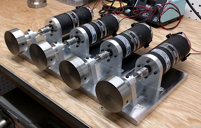
We now model the electromechanical systems from the laboratory, shown in figure 4.9. The system includes a brushed DC motor (Electrocraft 23SMDC-LCSS servomotor from Servo Systems), two shafts, a shaft coupler, two bearings, and a flywheel.

The motor’s datasheet specifications are given in . The mechanical subsystem’s inertia is dominated by the stainless steel flywheel with \(J_f = 0.324\cdot10^{-3}\) kg-m\(^2\). The bearing damping \(B_b\) is the most difficult parameter to determine. Let’s begin with the assumption that the combined bearing damping is \(B_b = 20\cdot10^{-6}\) N-m/(rad/s).
Linear graph model
A linear graph model is in order. An ideal voltage source drives the motor1—modeled as an ideal transducer with armature resistance \(R\) and inductance \(L\), given in . The ideal transducer’s rotational mechanical side (\(2\)) is connected to a moment of inertia \(J = J_m + J_f = 0.381\cdot10^{-3}\) kg-m\(^2\), dominated by the flywheel,2 and damping \(B\), which is the parallel combination of the internal motor damping of and the bearing damping \(B_b\), to yield \(B = 26.9\cdot 10^{-6}\) N-m/s\(^2\). We choose to ignore the flexibility of the coupler. Problem considers the same system but does not ignore the coupler’s flexibility. In general, shaft couplers have significant flexibility and, depending on the application, this may require consideration in the dynamic model.
a linear graph model of the electromechanical systems of fig:lab_electromechanical_stations.
State-space model
The normal tree can be constructed by the procedure from . The voltage source \(V_S\) is first included, followed by \(J\). Then exactly one edge of the ideal transducer must be selected, minimizing the number of T-types in the tree. We don’t really have a choice, in this case, because selecting edge \(2\) would create a loop, so we must select edge \(1\). Next, \(R\) is included. No more elements can be included without creating a loop, so we are finished.
We are now prepared to determine variables. The state variables are across variables of A-type tree branches and through variables of T-type links—so \(\Omega_J\) and \(i_L\), and the system is second-order (\(n=2\)). Clearly, the system’s input is the voltage source \(V_S\). We are interested in all the variables for the analysis in , so we choose them all for our outputs. In summary, then, the state, input, and output vectors are: \[\begin{gathered} \bm{x} = \begin{bmatrix} \Omega_J \\ i_L \end{bmatrix}, \ \bm{u} = \begin{bmatrix} V_s \end{bmatrix},\text{ and} \\ \bm{y} = \begin{bmatrix} \Omega_J & T_J & v_L & i_L & \Omega_B & T_B & v_R & i_R & v_1 & i_1 & \Omega_2 & T_2 & V_s & I_s \end{bmatrix}^\top. \end{gathered}\]
Let’s write some equations! Elemental are up first.
| \(J\) | \(\dfrac{d \Omega_J}{d t} = \dfrac{1}{J} T_J\) |
| \(L\) | \(\dfrac{d i_L}{d t} = \dfrac{1}{L} v_L\) |
| \(B\) | \(T_B = B \Omega_B\) |
| \(R\) | \(v_R = i_R R\) |
| \(1\) | \(\Omega_2 = v_1/TF\) |
| \(2\) | \(T_2 = -TF\, i_1\) |
the linear graph model for drawing contours.
Now, continuity and compatibility equations are developed by summing through-variables into contours. The three required contours—one for each of \(R\), \(1\), and \(J\)—can be drawn on figure 4.11. The three compatibility equations—one for each of \(L\), \(2\), and \(B\)—are found by “temporarily including” those links in the tree and summing across-variables around the loops created. Let’s write the equations.
| branch | continuity equation |
| \(R\) | \(i_R = i_L\) |
| \(1\) | \(i_1 = i_L\) |
| \(J\) | \(T_J = -T_2 - T_B\) |
| link | compatibility equation |
| \(L\) | \(v_L = -v_R+V_s-v_1\) |
| \(2\) | \(\Omega_2 = \Omega_J\) |
| \(B\) | \(\Omega_B = \Omega_J\) |
All that remains to form the state-space model is to eliminate variables that are neither states nor inputs from the elemental, continuity, and compatibility equations. Eliminating secondary variables by substituting the continuity and compatibility equations into the elemental equations, the following results.
| \(J\) | \(\dfrac{d \Omega_J}{d t} = -\frac{1} {J} (T_2 + T_B)\) |
| \(L\) | \(\dfrac{d i_L}{d t} = \frac{1} {L} (-v_R + V_s - v_1)\) |
| \(B\) | \(T_B = B \Omega_J\) |
| \(R\) | \(v_R = i_L R\) |
| \(1\) | \(v_1 = TF\, \Omega_J\) |
| \(2\) | \(T_2 = -TF\, i_L\) |
The last four equations allow us to eliminate the remaining undesirable variables to obtain the state model in the standard form3 $$\begin{align} \frac{d \bm{x}}{d t} &= A \bm{x} + B \bm{u} \\ \bm{y} &= C \bm{x} + D \bm{u} \end{align}$$ where $$\begin{align} A &= \begin{bmatrix}-B/J & TF/J\\ -TF/L & - R/L\end{bmatrix},\\ B &= \begin{bmatrix}0\\ 1/L \end{bmatrix},\\ C &= \begin{bmatrix}\Transpose{1 & 0\\- B & TF\\- TF & - R\\0 & 1\\1 & 0\\B & 0\\0 & R\\0 & 1\\TF & 0\\0 & 1\\1 & 0\\0 & - TF\\0 & 0\\0 & 1}\end{bmatrix}^\top,\text{ and } \\ D &= \begin{bmatrix}\Transpose{0\\0\\1\\0\\0\\0\\0\\0\\0\\0\\0\\0\\1\\0}\end{bmatrix}^\top. \end{align}$$
Often we can model our motor-driving source as ideal within an operating range. See for more details.↩︎
This is the sum of the inertia of the flywheel \(J_f = 0.324\cdot 10^{-3}\) kg-m\(^2\) and the rotor \(J_m = 0.0565\cdot 10^{-3}\) kg-m\(^2\). It might be worthwhile combining this with the inertia from the shaft and coupler to obtain a more accurate value, but the difference is likely negligible.↩︎
Here is the
rndfile for use with StateMint (statemint.stmartin.edu) to derive the state-space model from the elemental, continuity, and compatibility equations:Note that the “constraint equations” are the continuity and compatibility equations solved for primary variables.↩︎
Online Resources for Section 4.4
No online resources.